Desperately seeking squircles

In a famous 1972 interview, Charles Eames answered a short sequence of fundamental questions about the nature of design. Answering the first question, he defined design as “a plan for arranging elements to accomplish a particular purpose.” This principle holds true whether we’re selecting hues on a color wheel to achieve harmony or engineering the curves of a squircle for aesthetic smoothness.

His other answers are short, even quippy at times, but when asked about the role of constraint in design, he paused to give the longest and most considered response in the series: “Here is one of the few effective keys to the design problem: the ability of the designer to recognize as many of the constraints as possible; his willingness and enthusiasm for working within these constraints.”

Although I’m not a designer by trade — I’m an engineer who works on Figma, the web-based collaborative design tool — it’s easy to see how Eames’ remarks apply to my work as well. Instead of arranging UI elements to make products, I arrange mathematical concepts expressed in code to implement tools and features. And constraints of time, simplicity, maintenance, and even aesthetics play a similarly dominant role in my process.

One recent project highlights these parallels exceptionally well. I was tasked with somehow adding support for Apple’s quirkily-named ‘squircle’ shape to Figma — with little else to go on, I got to work doing research.

What unfolded was a mathematical odyssey, fraught with false starts, hidden problems, emergent constraints, exploration, tension and resolution. In short, it was a story every designer experiences, at some scale, almost every day.

To provide joy to math geeks like me and to illustrate how the design process unfolds when math is the medium, every step is presented below, from square one to shipping.

The squircle: Smooth operator

My story begins long before I started at Figma, on June 10th, 2013, the day Apple released iOS 7. There was something subtle about the update: the home screen’s app chiclets had a juicier, more organic feel. They’d gone from squares with rounded corners, to squircles (a portmanteau of ‘square’ and ‘circle’).

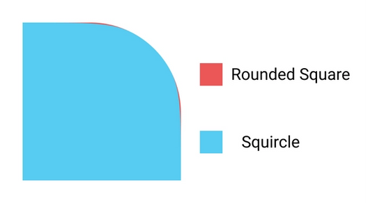
What is the difference, you ask? To be fair, it’s slight — A squircle begins as the old rounded square, but with some sandpaper applied to the part where the rounding begins on each side of each corner so the transition from straight to curved is less abrupt.

Articulating this using mathematical language is precise: The curvature of a squircle’s perimeter is continuous, whereas a rounded square’s is not. This may seem trivial, a cool story, but subconsciously it really makes a big impact: a squircle doesn’t look like a square with surgery performed on it; it registers as an entity in its own right, like the shape of a smooth pebble in a riverbed, a unified and elemental whole.

For a long time, industrial designers making physical objects have known how important curvature is to an object’s perception. Try taking a careful look at the corners of a Macbook, or at an old-school, wired earbud case under a desk lamp. Notice how difficult it is to find an orientation where the corners have harshly contrasting highlights.

This is the result of curvature continuity, and it’s very deliberately included in the design. It’s no surprise that Apple, with fingers uniquely in both the hard and software pies, eventually cross-pollinated their interface designs with industrial ideas by making their icons look like the physical things they produce.

From form to formula

Of course, at Figma we love iOS designers, and we feel our users should have the platform elements they need right at their fingertips. In order to give them access to this new shape while designing, we need to find a precise mathematical description so we can start figuring out how to build it into our tool.

Luckily, people have been asking this question for as long as iOS 7 has existed, and we are certainly not the first to walk this part of the journey! Fundamental initial work by Marc Edwards included a screenshot that indicated the icon shape was a particular generalization of an ellipse, called a superellipse. The following mathematical formula can describe circles, ellipses, and superellipses depending on how a, b, and n are chosen:

If you choose, say, n = 2, a = 5 and b = 3, you get a normal ellipse with a major axis of 5 oriented along x and a minor axis of 4 oriented along y. Keeping n = 2 and choosing a = b = 1 describes a perfect unit circle. However, if you choose a value for n that is bigger than two, the result is a superellipse — the rounded elliptical shape starts blending into the shape of its bounding rectangle, with the corners becoming perfectly sharp in the limit that n goes to infinity. Early suggestions tried describing Apple’s shape with n = 5. If you try it out, you’ll see it does look really close to what you’d find on a device running iOS 7+.

If this were the true description, we could just fit some reasonable number of Bézier segments to this shape and then do the delicate work of figuring out how to integrate this new concept into Figma. Unfortunately, though, careful follow-up efforts showed that the superellipse formula wasn’t quite right (however, these days true superellipses are used as icons in other contexts). In fact, for all choices of n in the equation above, there is a small but systematic discrepancy when compared with the real icon shape.

This is the first blind alley in the story: We have an elegantly simple equation for something that looks a lot like an iOS squircle, but it’s fundamentally incorrect. And we really do owe our users the real thing.

Making headway requires some serious effort, and again I’m glad to harvest what others have sown. One investigator, Mike Swanson of Juicy Bits, made a hypothesis which builds up the squircles’ corners using a sequence of Bézier curves, which he refined using a genetic algorithm to optimize similarity with the official Apple shape. The results he obtained turned out to be right on, as proven with Manfred Schwind’s excellent direct approach, which looks right at the iOS code which generates the icons. So we’ve got two different approaches yielding the same Bézier structure: iOS 7 Squircles were cracked and double checked by others, and we didn’t even have to calculate anything!

A spanner in the works

Two important details remain, preventing us from cloning the shape directly into Figma and moving on:

First, there is the surprising fact that the iOS version of the formula (at least at the time of investigation) was found to have some quirks — the corners aren’t exactly symmetrical, and one side has a minuscule straight segment which clearly doesn’t belong. We don’t want that because it complicates both code and tests, but removing the extra segment is easily handled by just mirroring the bug-free half of the corner.

Second, when flattening the aspect ratio of the real iOS rectangle shape, it abruptly changes from the squircle we’re focusing on to a totally different sort shape. This would be unpleasant for a designer, and takes a strong point of view about what shapes ‘should’ be used under certain circumstances.

The most natural and useful behavior when flattening a squircle is for the smoothing to gradually disappear until there’s no room left to “sand” the transition between the round and the straight parts of the corner. Flattening even further should reduce the rounded section’s corner radius, which is in line with how Figma behaves today. The Apple squircle formula is of little help to us here, because its smoothing is done in a fixed way: it gives no indication for how to get nearer to or further from the old rounded rectangle. What we really need is a parametrizable smoothing scheme, where some particular value of the parameter corresponds very closely to the Apple shape.

As an added bonus, if we can parametrize the smoothing process that transforms a rounded square into a squircle, we can likely apply the same process to other places where corner rounding happens in Figma: stars, polygons, and even corners in arbitrary vector networks drawn with the pen tool. Despite the complication, this is beginning to look like a much more complete and valuable feature than simply adding support for iOS 7 squircles would have been. We are now giving designers an infinite variety of new shapes to use in many situations, and one of them happens to correspond to the squircle icon shape that got us started in the first place.

Requiring that our squircle smoothing scheme be continuously adjustable yet conform to the iOS 7 shape at some comfortable point its adjustible range is the first emergent constraint in our story, and it’s a difficult one to satisfy. An analogous task would be for a dancer to take a single still image of a ballerina in mid-flight, then design a leap in such a way that a movie of her executing it reproduces the image exactly at a precise point in time. Which sounds freaking hard. So maybe some calculation will be necessary after all?

Power tools: Differential geometry of plane curves

Before diving into parameterizing squircles, let’s take a step back and dust off some formal tools that will help us analyze what’s going on. First of all, we need to settle on how we’ll describe a squircle. When discussing superellipses before, we used an equation involving x and y, where all the points (x, y) in the plane which satisfy the equation implicitly trace out the superellipse. This is elegant when the equation is simple, but real squircles are a patchwork of Bézier curves spliced together, which leads to unmanageably messy implicit equations.

We can deal with this complication by using a more explicit approach: take a single variable t, restrict it to a finite interval, and map each value which t can take on that interval to a distinct point on the squircle perimeter (Bézier curves themselves are almost always represented this way, in fact). If we concentrate on just one of the corners, thereby restricting our analysis to a curved line with a clear beginning and end, we can choose the mapping between t and the corner such that t = 0 corresponds to the beginning of the line, t = 1 corresponds to the end of the line, and smoothly sliding t between 0 to 1 smoothly traces out the round part of the corner. In mathematical language, we will describe our corner by the path r(t), which is structured as

where x(t) and y(t) are separate functions of t for the x and y components of r. We can think of r(t) as a kind of path history, say for a trip you’d take in your car. At every time t between when you begin and when you arrive, you can evaluate r(t) to get your car’s position along your route. From the path r(t) we can differentiate to get the velocity v(t) and acceleration a(t):

Finally, the mathematical curvature, which plays a starring role in our story, can in turn be expressed in terms of the velocity and acceleration:

But what does this formula really mean? Though it may look a bit complicated, curvature has a straightforward geometric construction, originally due to Cauchy:

1. The center of curvature C at any point P along the curve lies at the intersection of the line normal to the curve at P and another normal line taken infinitesimally close to P. (As a side note, the circle centered at C as constructed above is called the osculating circle at P, from the Latin verb osculare, meaning ‘to kiss’. 😙 Isn’t that great?)
2. The radius of curvature R is the distance between C and P.
3. The curvature κ is the inverse of R.

As constructed above, the curvature κ is nonnegative and doesn’t distinguish between rightward and leftward turns. Since we do care about this, we form the signed curvature k from κ by assigning a positive sign if the path is turning right, and a negative sign if the path is turning left. This concept too has an analogue in the car picture: at any point t, the signed curvature k(t) is just the angle through which the steering wheel has been turned at time t, with plus signs used for turns to the right and minus signs for turns to the left.

Geometry is king: Arc length parametrization

With curvature introduced, we have a last couple wrinkles to iron out. First, consider for a moment two cars driving along a squircle corner shaped route; one car keeps speeding up and then braking the entire way (🤢), while the other car smoothly speeds up then coasts down to a halt at the end. These two different ways of driving will yield very different path histories even though the exact same route was taken. We only care about the shape of the corner, not how any one driver negotiated it — so how can we separate the two? The key is to use not time to label the points in the history, but rather the cumulative distance traveled, or arc length. So instead of answering questions like ‘where was the car ten minutes into its trip?’, we’d rather answer ‘where was the car ten miles into its trip?’. This way of describing paths, the arc length parameterization, captures their geometry alone.

If we have some path history r(t) in hand, we can always extract the arc length s as a function of t from the path by integrating its speed, as follows:

If we can invert this relationship to find t(s), then we can substitute this for t in our path history r(t) to get the desired arc length parameterization r(s). The arc length parameterization of a path is equivalent to a path history made by a car driving at unit speed, so unsurprisingly the velocity v(s) is always a unit vector, and the acceleration a(s) is always perpendicular to the velocity. Consequently, the arc length parameterized version of curvature simplifies to just the magnitude of acceleration,

and we can tack on the appropriate right or left handed sign to form the signed curvature k(s). Most of the complication in the more general curvature definition was evidently there just to cancel out the non-geometric content in the path history. Curvature is, after all, a purely geometric quantity, so it’s really pleasing to see it look simple in the geometric parameterization.

Design the curvature, compute the curve

Now for the other wrinkle: we’ve just seen how to go from a path-history description of a curve r(t) to its arc length parameterization r(s), and how to extract the signed curvature k(s) from it. But can we do the reverse? Can we design a curvature profile and from it derive the parent curve? Let’s consider the car analogy again — suppose that as we were driving at constant unit speed along a route, we recorded the position of the steering wheel continuously throughout the journey. If we took that steering data and gave it later to another driver, they’d be able to reconstruct the route perfectly, so long as they played back the steering wheel positions properly and drove exactly the same speed. So we see intuitively that we have enough information to reconstruct the parent curve, but how does the computation look mathematically? It’s a little bit hairy, but it’s still possible, thanks to Euler, using the arc length parameterization — if we choose a coordinate system such that the curve starts at the origin and has its initial heading directed along the x axis, then x(s) and y(s) can be reconstructed from k(s) as follows:

Last, note the argument of the sine and cosine functions above: it is the integral of the signed curvature. Normally, the arguments supplied to trigonometric functions are angles measured in radians, and that turns out to be true in this case as well: the integral from a to b of the signed curvature is the heading at b minus the heading at a. Thus, if we start with a square and sand off the corner in whatever crazy way we want, then measure the curvature over the part we sanded and integrate up the result, we’ll always get π/2.

Squircles under the scalpel

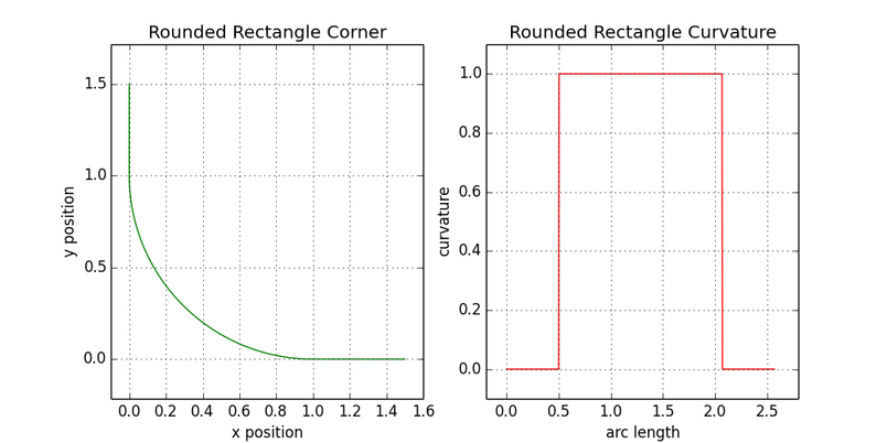
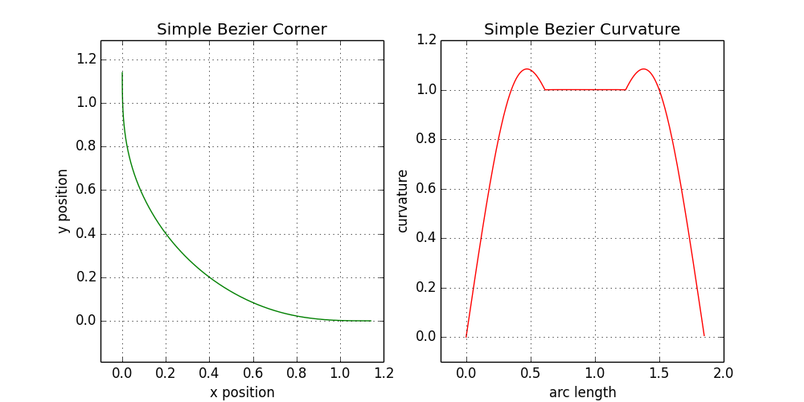
Now that we are wrinkle-free, let’s see what happens when we apply these analytical tools to some real shapes. We’ll start with a corner of a rounded rectangle which has a corner radius of one, plotting first the corner itself and then the curvature as a function of arc length:

We repeat this process now for the real Apple squircle corners to look at their curvatures, which is very different and very enlightening:

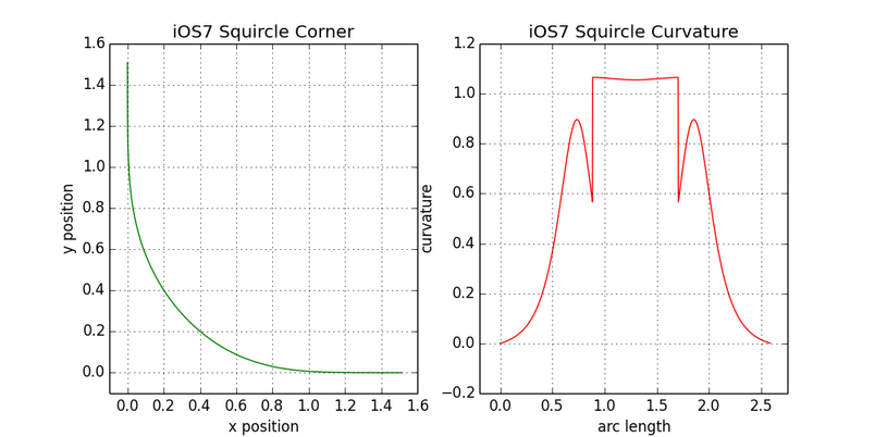
The curvature looks quite jagged, but this is not necessarily bad. As we’ll see later, there’s a tradeoff between having a smooth curvature plot and having a small number of Bézier curves, and the iOS corner only uses three. Generally, designers would rather deal with fewer Bézier curves at the expense of having a mathematically perfect curvature profile. These details aside, we can kind of squint at the plot on the right and see a general picture emerge: the curvature ramps up, flattens in the middle, and then ramps back down.

Breakthrough: Smoothing parameterized

Bingo! In that last observation lies the key to how we can parameterize the smoothing of our squircle corner. At zero smoothing, we want a curvature profile like the rounded rectangle: tabletop shaped. As smoothing slowly increases, we want the height of the tabletop to stay fixed while its cliff edges start turning into steep slopes, yielding an isosceles trapezoidal curvature profile (still with a total area of π/2, of course). As smoothing approaches its maximum, we want the flat part of the trapezoid to disappear, leaving us with a broad isosceles triangular profile whose peak height is that of the original tabletop.

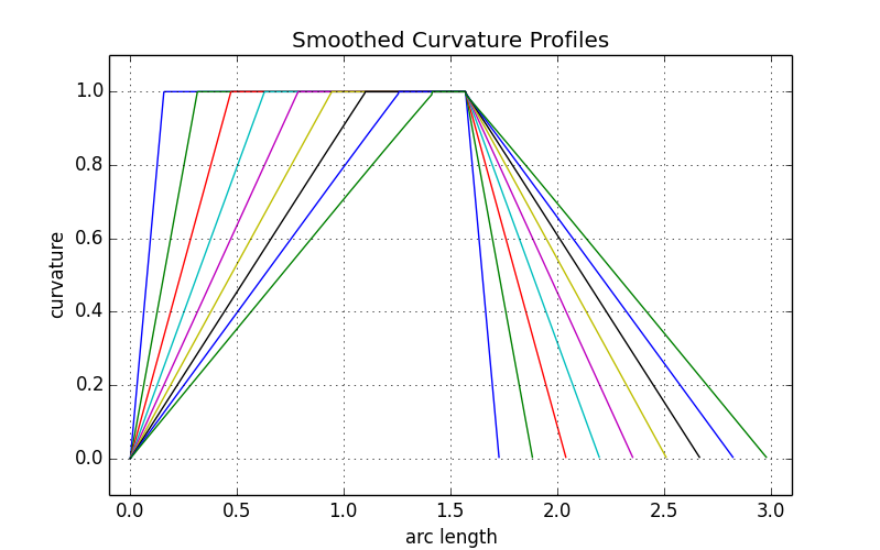
Let’s try to express this sketch of a curvature profile in mathematical terms, using ξ as a smoothing parameter which varies between zero and one. Foreseeing use with other shapes whose corners aren’t right angles, we also introduce the angle θ which is the turning angle of the corner — π/2 in the case of squares. Putting both together, we can define a piecewise function in three parts, one for the ramp up, one for the flat top, and one for the ramp down:

Notice that the first and third pieces (the ramps) disappear as ξ tends to zero, and that the middle piece (the flat top) disappears as ξ tends to one. We showed above how we can go from a curvature profile to a parent curve, so let’s try it out on the first equation above, which describes a line whose curvature starts at zero and steadily increases as we walk along it. We’ll do the easy interior integral first:

Great, so far so good! We can keep chugging along to form the next couple of integrals:

Alas, here we hit a bump, as these integrals aren’t quite as easy. If you have heard about the connection between trigonometric functions and exponentials, you might guess that these integrals are related to the error function, which can’t be expressed in terms of elementary functions. The same is true of these integrals. So what do we do? It is beyond the scope of this post to justify (see this math exchange post for a clue as to how you would), but in this case we can substitute in the Taylor expansions for sine and cosine, then swap the sum and the integral to obtain:

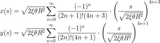
This looks nigh-impenetrable in its series form, so let’s take a step further and explicitly write out the first few terms in each series with all simplifying multiplication performed. This delivers the following few terms for the x and y parts of the shape:

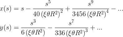
Apotheosis clothoid

This is a concrete result! We can actually plot this pair of equations (given some reasonable choices for ξ, θ and R) to get a path as a function of s. If we had access to arbitrarily many terms and could compute the sums, we’d see that as s increases, the curve begins to spiral in on itself, though this happens far from the domain we’re interested in, which is the flatter ramp-up section.

Echoing a sentiment from an earlier point in the post, we’re not the first to tread here, either. Owing to its linear curvature, which is very useful, many have stumbled on this curve in the past — it is known as an Euler spiral, cornu, or a clothoid, and it finds a lot of use in designing tracks for vehicles, including roads and roller-coasters.

Using the just the n < 10 part of the expansion as given in 8.5, we finally have all the pieces necessary to make our first artifact. The expansion represents the sloping (first) part of equation 8.2 — it’s easy to adapt it to the falling (third) part, and we’ll bridge these sloping portions with a circular arc for the flat (second) part. This method delivers a mathematically perfect squircle corner that exactly follows the curvature design we first introduced in equations 8.2. Here is the curvature analysis performed for a clothoid squircle corner with ξ = 0.4:

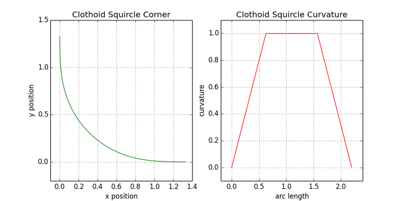
Though it feels good to have obtained this elegant shape, we must realize this is only an ideal version. This exact shape won’t work for several reasons, first among which is the fact that the center of curvature of the circular portion moves as a function of the smoothing parameter ξ — ideally, it would remain fixed.

More importantly, the power of the arc length s in the terms we’ve kept to produce the plots can be as high as nine. In Figma, continuous paths must be representable by cubic Bézier curves (of which quadratic Bézier curves and lines are special cases) and this limits us to keeping only cubic and lower order terms. This means that the series above for x(s) and y(s) must each be truncated to a single term. It’s hard to have much confidence that such a drastic truncation will retain the properties we like.

Sadly, discarding higher-order terms is not sufficient — the resulting construction performs very poorly when ξ is large. We can see this below in the figure drawn for ξ = 0.9:

This shape is clearly unusable. It seems three orders isn’t enough to keep the curvature increasing throughout the ramp up and ramp down sections of the parameterization, meaning that we have a ton of accumulated error by the time we get to the circular section. Sadly, this means that all of our clothoid results are unusable, and we have to go back to the drawing board.

Nothing gold can stay

Let’s take a step back, consider our constraints again, and try to extract what we can from the previous efforts before heading off in a new direction.

First, we know that the perfect clothoid construction has exactly the curvature profile we need, but the center of curvature of the central circular section changes location as a function of the smoothing parameter ξ. This is undesirable because our current on-canvas rectangle rounding UI uses a dot right at the center of curvature which a user can drag to set the corner radius. It might feel a bit weird if that dot moved as the smoothing varied. Also, the iOS shape’s central section is right where it would be if it were just a rounded rectangle, further implying total independence of the center’s location from ξ. So we can keep the same basic curvature design goal and add the constraint that the circular section keep a fixed center of curvature as ξ varies.

Second, we know that designers don’t want the construction of the squircle corner to be too complicated. Apple’s squircle (after removing the weird tiny straight part) has only one Bézier curve connecting its circular section to the incoming edge, so maybe we can construct the same type of thing?

Thirdly, we have a somewhat arcane technical constraint which isn’t apparent at the outset, but that becomes a major implementation issue. To approach this, let’s consider a square, 100px by 100px, which has vanilla corner rounding applied for a corner radius of 20px. This means that each side of the square’s perimeter has 60px of straight track. If we flatten the square into a squashed rectangle so that it’s 80px by 100px, then the straight section of the short side will be only 40px long. What happens when we flatten the square so much that we run out of straight section? Or if we flatten it more, so that the rectangle is, say, 20px by 100px? Figma’s present behavior is to figure out the largest value of corner rounding we have room to apply and then draw the shape using that instead. Our 20px by 100px rectangle would thus have 10px of rounding applied.

Any smoothing process we might use to create a squircle will eat up even more of the straight edge than simple rounding does. Imagine the case above again, a 100px by 100px rectangle, apply 20px of rounding, and then apply some smoothing procedure which removes 12 more pixels from the straight sides. This leaves us with a 36px budget in the straight section for flattening. What happens when flattening the rectangle to 60px by 100px? It seems almost obvious, by analogy, that we should back off the smoothing until the budget is balanced and the straight portion is exactly consumed. But how do we compute the value of ξ which satisfies a specific pixel consumption budget? We must be able to do this quickly or we can’t implement the feature.

Again, this problem has a very precise mathematical articulation: If smoothing corners with radius R and parameter ξ consumes p pixels, then the function p(R,ξ) must be invertible to ξ(R,p). This is a somewhat hidden constraint which would also have ruled out a high order clothoid series solution.

Finally, we have a usability constraint, which is that changing the smoothing should actually do something perceptible to the shape. If we yank the smoothing parameter ξ back and forth between zero and one, it better make a visible difference! Imagine we did all this work for something that people can barely see — it’s unacceptable. This is fundamentally a requirement of usefulness, and as such it’s obviously the strongest constraint.

Keep it simple, squircle

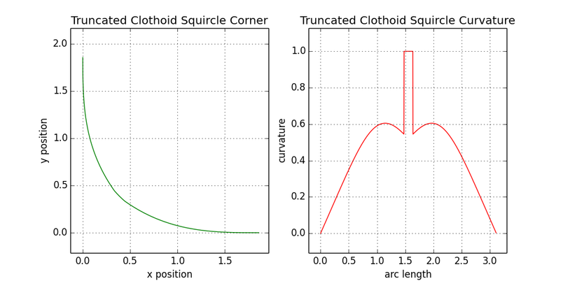
Let’s try the most direct thing we can think of that meets the constraints listed above and just try to pick a single parameterized Bézier curve that takes the circular portion and links it up to the straight side. The figure below shows a type of Bézier curve suitable for this purpose:

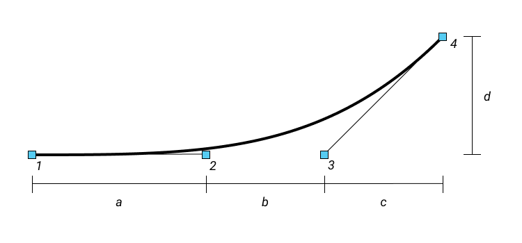
A few of its properties merit further explanation. First, control points 1, 2 and 3 all fall in a line. This ensures that the curvature at point 1, which connects to the straight part of the squircle, is exactly zero. Generally speaking, if we define a coordinate system and associate point 1 with P1, point 2 with P2, and so on, the curvature at point 1 is given by:

We can see, reassuringly, that the cross product vanishes when points 1–3 are collinear. This same formula can be applied to point 4 by labeling in reverse; doing so and plugging in the geometry and the labels in the figure gives the following for the curvature there:

Ideally, this would be the same as the curvature of the circular section, or 1/R, which provides us one more constraint. Finally, the values of c and d are fixed by the fact that the end of this curve has to meet the circular portion and be tangent to it where it joins, which means the curvature constraint above just gives us the value of b:

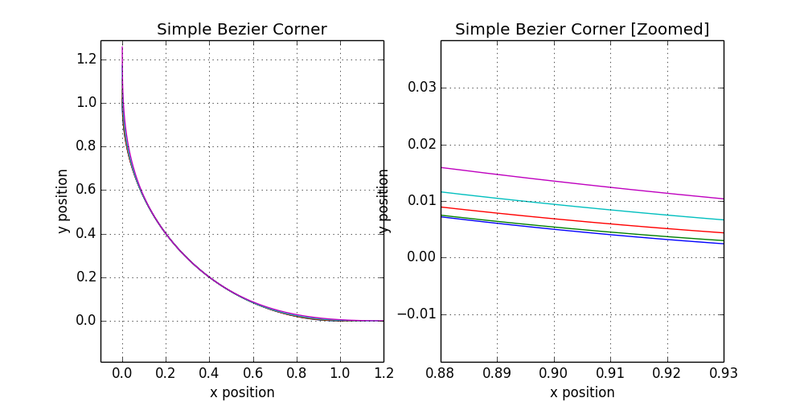
If we find it important to preserve the initial linear increase in curvature (which the ideal clothoid solution featured at point 1) we can set a equal to b, which fixes all of the points on the Bézier curve and gives us a potential solution. Using these observations, we construct a simple Bézier squircle below using a smoothing of ξ = 0.6:

This looks pretty good, and it takes a lot of cues from the original clothoid calculation. Unfortunately, the variation over the full range, from ξ = 0 to 1 only makes a very subtle difference in the corner shape. Here we’ll show the corner at two zoom levels, with curves for ξ = 0.1, 0.3, 0.5, 0.7, and 0.9 shown in different colors:

This is a barely noticeable effect despite its nice mathematical properties. It’s certainly closer to being a product than the curve we got by truncating the clothoid series that we considered previously. If we could only tweak the formula a little bit to get some more variation!

Small strokes of sqluck

We can take one more small step back to figure out how to proceed. Recalling that we need an invertible relationship between pixels consumed in smoothing and the smoothing parameter ξ, we can focus initially on this mapping, make it as simple as possible, and see what comes out when we try to make a parametrization of squircles from it.

We know something already about how simply rounding the corners consumes pixels. I won’t walk through the trigonometry necessary, but taking a corner of opening angle θ and rounding it to have a radius of R pixels will consume q pixels of the edge from the apex of the corner, with q given as follows:

What if we choose p(R,ξ) based on q in just the simplest possible way, something like:

All this means is that our maximum smoothing setting will consume again the length of segment that we consumed in rounding normally. Making this choice would fix the quantity a + b from the figure above. Recall that in any circumstance c and d are firmly fixed, so fixing a + b means there is one final decision to make: how large is a relative to b? Again, if we make the simplest choice, namely a = b, we have determined another modified Bézier parameterization, whose corners and curvatures we show below:

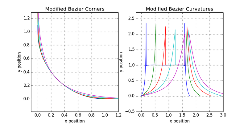
That visual variation looks promising! The curves look attractive, sanded in a way. However the curvature profile looks pretty rough. If we could just make it a bit less spiky, it might be a serious contender for a product. Despite the poor curvature profile, even this simple family of shapes has a member that looks extremely similar to the Apple version of the squircle, almost close enough to put in front of our users without a bad conscience.

Now we turn to the curvature profile, our last outstanding problem. Rather than splitting the difference evenly between a and b as we did above, why don’t we give two thirds of the interval to a and the remaining third to b? This will throttle the curvature from increasing too quickly, reducing the long tails on the curvature profile and cutting at the spikes. This modification results in the following shapes:

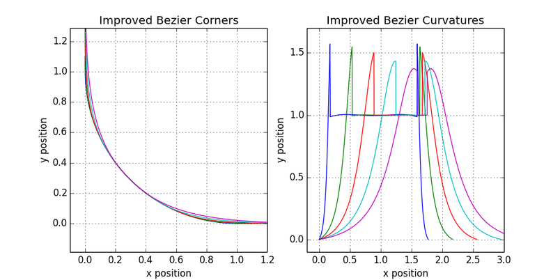
The curvature profiles are much improved, the visual degree of variation is still enough for this to be a useful product, ξ = 0.6 just about nails the iOS shape, and the nice visual character of the curves which this stunningly simple approach generates is retained. So we must ask the question — what’s blocking this from becoming the product? Nothing.

Watching the ship sail

It’s useful here, at the end, to reflect on the process itself. Something I see borne out repeatedly in this story is the power and effectiveness of trying the simplest possible thing. Doing so will, in the worst case, give a baseline for comparison if the simplest thing ends up not working out. Evaluating it in a serious way also shines a light on the most important things we need to consider when refining the approach and moving forward. And in the best cases, like ours, the simplest thing happens to be pretty good already!

Lastly, there is a meditation on the difference between a good product and a perfect one. I feel some pangs of embarrassment writing this that I was unable to come up with a better curvature profile. I’m sure I could have given more time — there are many avenues left to explore. Intellectually, it’s somewhat unsatisfying to have gotten such a beautiful result as the clothoid series but not to have been able to at least see a reflection of that in the spline we shipped in the end. But there’s also the wider context — the constraints of time when working at a small company are very real — and a design which violates these cannot be considered good.

If this type of problem resonates with you, we’re hiring!